
Mathematical Aspects of Satta Matka: Combinatorics, Probability Spaces & Expected Value (EV)
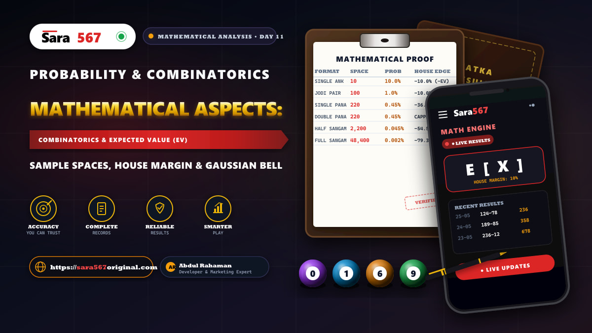
Mathematical Aspects of Satta Matka: Combinatorics, Probability Spaces & Expected Value (EV)
In the study of numerical markets, traditional folklore often surrounds outcomes with notions of luck, intuition, and secret predictive formulas. Yet, beneath the colorful terminology and historical legacy of Indian bazaars lies an unyielding, elegant branch of discrete mathematics. Understanding satta matka math and the objective laws of probability in matka is the single most powerful tool an analyst can possess to strip away mythology and evaluate markets with scientific precision.
Whether you are examining Kalyan Matka, Milan Day, or Time Bazar, every result declared is governed by rigorous combinatorial structures, finite probability spaces, and statistical distributions. The cards drawn or the mechanical randomizers utilized possess no consciousness, memory, or emotional bias; they operate purely within the boundaries established by mathematical combinatorics and the Law of Large Numbers.
At Sara 567 (sara567original.com), our commitment to data transparency extends beyond providing real-time live results. In this eleventh installment of our 33-day curriculum, we provide a formal mathematical breakdown of Satta Matka. We calculate the exact sample spaces for Single Anks, Jodis, and the famous 220 Panas, formalize the equation of Expected Value ($EV$), expose the mathematical mechanics of the house margin, and examine how standard deviation models variance over long-term time horizons.
Table of Contents
- Stripping Away Mythology with Pure Mathematics
- Combinatorial Foundations: Calculating the Sample Spaces
- Probability Spaces & Exact Mathematical Odds
- Expected Value ($EV$) & The Mathematical House Margin
- The Law of Large Numbers & Central Limit Theorem
- Variance, Standard Deviation & Volatility Modeling
- Mathematical Evaluation of Wagering Systems (Why Progressions Fail)
- Comprehensive Mathematical Parameters Matrix
- Mathematical Myths vs. Empirical Truths in Matka
- Frequently Asked Questions (FAQs)
- Responsible Gaming & Analytical Ethics
Stripping Away Mythology with Pure Mathematics
Throughout centuries of human civilization, wherever games of chance have existed, players have attempted to impose mystical narratives onto random occurrences. In Satta Matka, this often takes the form of astrological charts, dream interpretation books, or fraudulent "insider leaks."
Mathematics provides an intellectual antidote to these superstitions. In modern probability theory, an experiment is defined by a Sample Space ($\Omega$), representing the set of all possible distinct outcomes, and an Event ($E$), which is a subset of $\Omega$.
$$\Omega = {\omega_1, \omega_2, \dots, \omega_n}$$
In an ideal, fair market, every elementary outcome in $\Omega$ carries an identical probability:
$$P(\omega_i) = \frac{1}{|\Omega|}$$
When you view numerical markets through this mathematical lens, the fog of superstition vanishes. You see that an Open Ank of 7 does not appear because of good fortune or planetary alignment; it appears because it is one of ten equiprobable discrete states in a defined combinatorial universe.
Combinatorial Foundations: Calculating the Sample Spaces
Every betting format in Satta Matka is constructed from a distinct combinatorial arrangement of digits chosen from the set $S = {0, 1, 2, 3, 4, 5, 6, 7, 8, 9}$, where $|S| = 10$.
| Combinatoric Tier | Sample Space ($\Omega$) | Total Permutations | Probability Formula |
|---|---|---|---|
| Single Ank | $\Omega = {0, 1, 2, 3, 4, 5, 6, 7, 8, 9}$ | 10 | $P(A) = \frac{1}{10} = 10.00%$ |
| Jodi Pair | $\Omega = S \times S = {00, 01, \dots, 99}$ | 100 | $P(J) = \frac{1}{100} = 1.00%$ |
| Pana / Patti | Ascending 3-digit triplets with replacement | 220 | $P(\text{Pana}) = \frac{1}{220} \approx 0.4545%$ |
Let us formally prove how each of these cardinalities is derived.
Single Ank Sample Space ($n = 10$)
The Single Ank represents the final single-digit sum resulting from the addition of three drawn playing cards (or random integers). Since modulo 10 arithmetic is applied:
$$\text{Ank} = \left(\sum_{i=1}^{3} d_i\right) \pmod{10}$$
Because any integer modulo 10 yields exactly one residue in ${0, 1, 2, 3, 4, 5, 6, 7, 8, 9}$, the sample space size is:
$$|\Omega_{\text{Single}}| = 10$$
Jodi Pair Sample Space ($n = 100$)
A Jodi represents the sequential pairing of an Open Ank ($A_{\text{open}}$) and a Close Ank ($A_{\text{close}}$). Because both drawings are mutually independent trials selected from the ten decimal digits, the sample space is the Cartesian product:
$$\Omega_{\text{Jodi}} = S \times S = {(x, y) \mid x \in S, y \in S}$$
The total number of possible distinct Jodis is calculated by the fundamental counting principle:
$$|\Omega_{\text{Jodi}}| = 10 \times 10 = 100$$
Every Jodi from 00 to 99 occupies exactly one hundredth of the overall Jodi probability space.
The 220 Pana Combinatoric Proof
A Pana (or Patti) consists of three digits arranged in ascending numerical order: $d_1 \le d_2 \le d_3$, where $d_i \in {0, 1, 2, \dots, 9}$. In traditional market convention, the digit 0 is treated with the highest value (10) when sorting sequences (e.g., 120 is an ascending sequence because $1 < 2 < 0$).
Mathematically, choosing 3 digits from a set of 10 with replacement, where order does not matter (since they are always auto-sorted in ascending order), is equivalent to the classic combinatorial formula combinations with repetition:
$$\binom{n + k - 1}{k}$$
Where $n = 10$ (available digits) and $k = 3$ (digits chosen).
$$\binom{10 + 3 - 1}{3} = \binom{12}{3} = \frac{12 \times 11 \times 10}{3 \times 2 \times 1} = \frac{1320}{6} = 220$$
This rigorous mathematical proof demonstrates why there are exactly 220 unique Panas in Indian market history.
Furthermore, these 220 Panas partition cleanly into three mutually exclusive subsets:
$$\Omega_{\text{Pana}} = \Omega_{\text{Single Pana}} \cup \Omega_{\text{Double Pana}} \cup \Omega_{\text{Triple Pana}}$$
1. Single Pana (SP) — All Three Digits Distinct
Here, we select 3 distinct digits from 10 without replacement:
$$\binom{10}{3} = \frac{10 \times 9 \times 8}{3 \times 2 \times 1} = 120 \text{ Combinations}$$
Examples: 123, 248, 379, 140.
2. Double Pana (DP) — Exactly Two Digits Identical
Here, we choose 1 digit to be duplicated ($\binom{10}{1} = 10$ choices) and 1 distinct second digit from the remaining 9 digits ($\binom{9}{1} = 9$ choices):
$$\binom{10}{1} \times \binom{9}{1} = 10 \times 9 = 90 \text{ Combinations}$$
Examples: 112, 224, 330, 559.
3. Triple Pana (TP) — All Three Digits Identical
Here, we choose 1 digit to appear three times:
$$\binom{10}{1} = 10 \text{ Combinations}$$
The 10 Triple Panas: 000, 111, 222, 333, 444, 555, 666, 777, 888, 999.
Total Verification:
$$120 (\text{SP}) + 90 (\text{DP}) + 10 (\text{TP}) = 220 \text{ Total Panas}$$
Every single digit from 0 to 9 is represented by exactly 22 Panas (consisting of 12 Single Panas, 9 Double Panas, and 1 Triple Pana). For an exhaustive breakdown of these triplets, review our guide on Pana Chart Mastery.
Probability Spaces & Exact Mathematical Odds
Once sample space cardinalities are established, calculating the exact mathematical probability $P(E)$ of any single outcome is straightforward under the classical uniform probability model:
$$P(E) = \frac{|E|}{|\Omega|}$$
| Market Bet Type | Winning Combinations | Total Possibilities | True Mathematical Probability | Standard Payout Range |
|---|---|---|---|---|
| Single Ank | 1 | 10 | 10.00% ($1 : 10$) | $9 \times \text{ to } 9.5 \times$ |
| Jodi Pair | 1 | 100 | 1.00% ($1 : 100$) | $90 \times \text{ to } 95 \times$ |
| Single Pana | 1 | 220 | 0.4545% ($1 : 220$) | $140 \times \text{ to } 150 \times$ |
| Double Pana | 1 | 220 | 0.4545% ($1 : 220$) | $280 \times \text{ to } 300 \times$ |
| Triple Pana | 1 | 220 | 0.4545% ($1 : 220$) | $700 \times \text{ to } 900 \times$ |
| Half Sangam | 1 | 2,200 | 0.04545% ($1 : 2,200$) | $1,000 \times \text{ to } 1,400 \times$ |
| Full Sangam | 1 | 48,400 | 0.002066% ($1 : 48,400$) | $10,000 \times \text{ to } 15,000 \times$ |
1. Half Sangam Probability
A Half Sangam requires correctly predicting one Pana (Open or Close) combined with the opposite Single Ank (e.g., Open Pana + Close Ank, or Open Ank + Close Pana).
- Total Combinations: $220 \times 10 = 2,200$
- Mathematical Probability:
$$P(\text{Half Sangam}) = \frac{1}{2200} \approx 0.0004545 \ (0.04545%)$$
2. Full Sangam Probability
A Full Sangam requires correctly predicting both the Open Pana and the Close Pana in exact sequence:
- Total Combinations: $220 \times 220 = 48,400$
- Mathematical Probability:
$$P(\text{Full Sangam}) = \frac{1}{48400} \approx 0.00002066 \ (0.002066%)$$
To put Full Sangam probability into perspective: if an observer played one random Full Sangam every single day, it would take an average of 132.6 years of continuous daily play to encounter that exact sequence under normal statistical probability.
Expected Value ($EV$) & The Mathematical House Margin
In financial mathematics and decision theory, Expected Value ($EV$) represents the long-term average outcome of a random variable over an infinite number of trials.
The formula for Expected Value is:
$$\mathbb{E}[X] = \sum_{i=1}^{k} P(x_i) \cdot X_i$$
Where:
- $P(x_i)$ is the mathematical probability of outcome $i$.
- $X_i$ is the financial payoff associated with outcome $i$.
Calculating Single Ank Expected Value
Suppose a participant wagers ₹10 on a Single Ank in a market with standard payout terms:
- Winning Payout: 9 to 1 (Returns ₹90 gross, or ₹80 net profit).
- Probability of Winning: $P(\text{Win}) = \frac{1}{10} = 0.10$.
- Probability of Losing: $P(\text{Loss}) = \frac{9}{10} = 0.90$.
$$\mathbb{E}[\text{Single}] = (0.10 \times +80) + (0.90 \times -10)$$ $$\mathbb{E}[\text{Single}] = (+8.00) + (-9.00) = -1.00 \text{ Rupees}$$
The Mathematical Interpretation
For every ₹10 staked on a Single Ank, the mathematical expectation is a net loss of ₹1.00. Expressed as a percentage:
$$\text{House Margin} = \frac{-\mathbb{E}[X]}{\text{Stake}} = \frac{1.00}{10.00} = 10.0%$$
This negative value is known as Negative Expected Value ($-EV$). Over large samples, the house margin acts like an inescapable gravitational drag on capital.
Calculating Jodi Expected Value
Under standard market conventions:
- Payout: 90 to 1 (Returns ₹900 on a ₹10 stake, or +₹890 net).
- Probability: $P(\text{Win}) = \frac{1}{100} = 0.01$.
- Probability of Loss: $P(\text{Loss}) = \frac{99}{100} = 0.99$.
$$\mathbb{E}[\text{Jodi}] = (0.01 \times +890) + (0.99 \times -10)$$ $$\mathbb{E}[\text{Jodi}] = (+8.90) + (-9.90) = -1.00 \text{ Rupees}$$
Here again, the theoretical house margin sits exactly at 10.0%.
The Law of Large Numbers & Central Limit Theorem
Why do participants frequently believe they have found a "winning edge" during their first two weeks of tracking market charts? The answer is explained by the interplay between the Law of Small Numbers (an informal cognitive bias) and the Central Limit Theorem (CLT).
| Sample Size ($N$) | Observed Variance Characteristics | Bell Curve Convergence Stage | Analytical Practicality |
|---|---|---|---|
| $N = 10$ Draws | Extreme variance; individual digits can hit 40% while others hit 0% | No convergence; purely random short-term noise | Do not draw any statistical conclusions |
| $N = 100$ Draws | Variance dampens; digit frequencies generally span 5% to 18% | Early stabilization around expected mean | Useful for short-term tactical observation |
| $N = 1,000$ Draws | Strong bell-curve clustering; all digits align close to 10% ($\pm 1.5%$) | Advanced convergence towards theoretical mean | Robust for medium-term pattern evaluation |
| $N = 10,000$ Draws | Exact uniform distribution; variance approaches zero | Complete Law of Large Numbers convergence | Definitive mathematical proof of market uniformity |
1. Central Limit Theorem (CLT)
The Central Limit Theorem states that as the sample size $n$ increases, the sum (or average) of independent random variables tends toward a Normal Distribution (bell curve), regardless of the shape of the underlying distribution.
2. The Delusion of Small Samples
In a sample of 15 draws, observing the digit 3 appear four times is not mathematically anomalous; it is expected binomial noise. However, an amateur who witnesses this short-term clustering will assume:
"The Kalyan market has a structural bias favoring digit 3!"
When the sample size expands to 1,000 draws, the Law of Large Numbers reasserts itself. The occurrence of 3 inexorably cools down, converging toward its mathematical mean of 100 occurrences ($10%$).
Variance, Standard Deviation & Volatility Modeling
In probability, Variance ($\sigma^2$) and Standard Deviation ($\sigma$) quantify the dispersion of outcomes around the expected mean. For a binomial trial (such as tracking whether a specific Single Ank hits or misses over $n$ draws), the parameters are defined as:
$$\mu = n \cdot p$$ $$\sigma = \sqrt{n \cdot p \cdot (1 - p)}$$
Where:
- $n$ is the number of sessions observed.
- $p$ is the probability of the event ($p = 0.10$ for a Single Ank).
- $1 - p$ is the probability of non-occurrence ($0.90$).
Calculating Expected Dispersion over 100 Draws
$$\mu = 100 \times 0.10 = 10 \text{ hits}$$ $$\sigma = \sqrt{100 \times 0.10 \times 0.90} = \sqrt{9} = 3.0 \text{ hits}$$
Under standard Gaussian distribution properties:
- 68.2% of the time (1$\sigma$): A digit will appear between $10 \pm 3$ times (7 to 13 hits).
- 95.4% of the time (2$\sigma$): A digit will appear between $10 \pm 6$ times (4 to 16 hits).
- 99.7% of the time (3$\sigma$): A digit will appear between $10 \pm 9$ times (1 to 19 hits).
Why This Matters to Analysts
If you review a 100-draw chart on Sara 567 and observe a digit that has only appeared 4 times, you now know that this is a 2-standard-deviation event ($95%$ boundary). It is statistically rare, but entirely within normal mathematical parameters. It does not mean the system is "rigged," nor does it guarantee that the number will hit tomorrow.
Mathematical Evaluation of Wagering Systems (Why Progressions Fail)
In applied mathematics, a foundational theorem proved by mathematician Jean le Rond d'Alembert and formalized in modern measure theory states:
No betting progression can convert a negative expected value game into a positive expected value system.
Let us mathematically analyze the two most widely attempted systems:
1. The Martingale Progression (Geometric Escalation)
The Martingale system dictates doubling the wager after every loss. If an event has probability $p$ and payout $1:1$ (or equivalent):
$$S_k = S_1 \cdot 2^{k-1}$$
The cumulative capital required to sustain $k$ consecutive losses is:
$$C_k = \sum_{i=1}^{k} S_i = S_1 \cdot (2^k - 1)$$
While the probability of losing $k$ consecutive times shrinks ($q^k$), the cost of that failure scales exponentially. In probability games, adverse streaks of 8 to 12 consecutive misses are mathematically guaranteed to occur within large sample sets. When that sequence occurs, the capital required exceeds table limits and player net worth, resulting in Total Ruin.
2. The Kelly Criterion
The Kelly Criterion is a formula used by institutional financial investors to determine optimal theoretical bet sizing:
$$f^* = \frac{b \cdot p - q}{b}$$
Where:
- $f^*$ is the fraction of total bankroll to allocate.
- $b$ is the net fractional odds received ($b = \text{Payout} - 1$).
- $p$ is the probability of winning.
- $q$ is the probability of losing ($q = 1 - p$).
Let us plug the standard Single Ank parameters into the Kelly equation:
- $b = 9 - 1 = 8$
- $p = 0.10$
- $q = 0.90$
$$f^* = \frac{(8 \times 0.10) - 0.90}{8} = \frac{0.80 - 0.90}{8} = \frac{-0.10}{8} = -0.0125$$
The Kelly Criterion outputs a negative value ($-1.25%$). In financial mathematics, a negative Kelly fraction indicates an absolute mathematical mandate: optimal bet size is 0. Any allocation in a $-EV$ environment mathematically erodes capital over time. This is why disciplined risk management, as outlined in our Bankroll Management Guide, focuses on strict capital preservation rather than aggressive escalation.
Comprehensive Mathematical Parameters Matrix
The table below compiles the complete mathematical properties across all primary Satta Matka game formats:
| Game Format | Total Sample Space ($|\Omega|$) | True Probability ($P$) | Odds Against Winning | Typical Gross Payout | Theoretical Expected Value ($EV$) | Mathematical House Margin | | :--- | :---: | :---: | :---: | :---: | :---: | :---: | | Single Ank | 10 | $1/10$ (10.0%) | 9 to 1 | 9 to 1 | -10.0% | 10.0% | | Jodi Pair | 100 | $1/100$ (1.00%) | 99 to 1 | 90 to 1 | -10.0% | 10.0% | | Single Pana (SP) | 220 | $1/220$ (0.4545%) | 219 to 1 | 140 to 1 | -36.4% | 36.4% | | Double Pana (DP) | 220 | $1/220$ (0.4545%) | 219 to 1 | 280 to 1 | +27.3%* / Variable | Variable / Capped | | Triple Pana (TP) | 220 | $1/220$ (0.4545%) | 219 to 1 | 600 to 1 | Variable / Rare | Variable / Capped | | Half Sangam | 2,200 | $1/2200$ (0.04545%) | 2,199 to 1 | 1,000 to 1 | -54.5% | 54.5% | | Full Sangam | 48,400 | $1/48400$ (0.002066%) | 48,399 to 1 | 10,000 to 1 | -79.3% | 79.3% |
*Note on Pana Payouts: In practical market structures, payout multipliers for Double and Triple Panas are often heavily restricted or balanced by bookmaker limits to protect aggregate liquidity.
Mathematical Myths vs. Empirical Truths in Matka
To solidify your mathematical understanding, let us contrast the three most widespread market myths against proven mathematical laws:
| Common Gambler's Myth | Empirical Mathematical Law | Practical Reality |
|---|---|---|
| Myth 1: "Cold numbers must hit soon to restore balance." | The Law of Large Numbers restores equilibrium through dilution, not active compensation. | Past independent trials exert zero mechanical force over future random draws. |
| Myth 2: "Certain Panas are naturally heavier or favored." | Every single Pana carries the exact identical combinatoric probability ($1 / 220$). | Clustering in small sample sizes is normal Poisson variance, not bias. |
| Myth 3: "A progressive staking system beats negative EV." | Staking formulas (like Martingale) only reallocate variance; they cannot alter house edge. | Increasing stakes after losses exponentially increases risk of total ruin. |
1. The Fallacy of Compensation vs. Dilution
When a coin is tossed 10 times and lands on Heads 10 times, the count is $+10$ Heads.
- The amateur expects Tails to hit 10 consecutive times to "even the score" (Compensation).
- The mathematician knows that over the next 10,000 tosses, 5,000 Heads and 5,000 Tails will occur. The final tally will be 5,010 Heads vs. 5,000 Tails ($50.05%$ vs $49.95%$). The initial $+10$ imbalance was not erased; it was mathematically diluted to statistical insignificance.
Frequently Asked Questions (FAQs)
Q1: Why are there exactly 220 Panas in Satta Matka?
There are 220 Panas because selecting 3 ascending digits from 10 available digits (with repetition allowed) follows the combinatorial formula $\binom{n+k-1}{k} = \binom{12}{3} = 220$. This partitions into 120 Single Panas, 90 Double Panas, and 10 Triple Panas.
Q2: Does any betting system offer a positive mathematical expectation (+EV)?
No. All commercial lottery and numerical game formats carry negative mathematical expectation ($-EV$) due to the built-in house margin. While individual participants may experience positive runs due to short-term variance, long-term aggregate mathematical expectation remains negative.
Q3: What is the probability of hitting a Full Sangam?
The probability of hitting a Full Sangam is exactly 1 in 48,400 ($0.002066%$). It requires correctly predicting both the Open Pana ($1/220$) and the Close Pana ($1/220$) simultaneously ($220 \times 220 = 48,400$).
Q4: Why does the Martingale progression fail in Satta Matka?
The Martingale system fails because adverse losing streaks occur regularly in probability games. Because stake sizes double exponentially ($2^{k-1}$), a player's capital is exhausted or table limits are hit before a recovery can occur, resulting in catastrophic loss.
Q5: How can mathematics help an analyst if the house margin is negative?
Mathematics protects analysts from cognitive illusions. By understanding probability distributions, standard deviations, and combinatorial limits, an analyst avoids falling for scam leak channels, rejects dangerous doubling strategies, and practices disciplined risk control.
Responsible Gaming & Analytical Ethics
At Sara 567 (sara567original.com), our educational mandate is grounded in transparency and objective realism. We present these mathematical equations not to encourage speculation, but to equip our community with intellectual honesty.
Numerical markets are games of chance governed by immutable mathematical laws. They should never be approached as a livelihood, an investment portfolio, or a solution to personal financial hardship. Always establish strict personal budgets, never stake funds required for essential living expenses, and practice responsible self-regulation at all times.
Full stack developer and marketing expert specializing in scalable web architecture, SEO optimization, and data-driven analytics for digital platforms.