
Understanding Result Patterns in Satta Matka: The Complete Guide to Chart Trends & Statistical Analysis
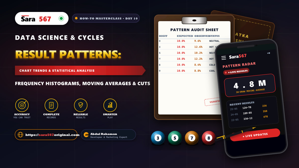
Understanding Result Patterns in Satta Matka: The Complete Guide to Chart Trends & Statistical Analysis
Across decades of market history, the pursuit of satta matka patterns and historical result trends has remained the central obsession of analysts, statisticians, and recreational players alike. Whenever numbers are recorded in chronological sequence—whether in Kalyan Matka, Milan Day, or Time Bazar—the human eye naturally seeks order. We observe clusters of repeating digits, recurring Jodi families, and rhythmic cyclical oscillations that seem to hint at underlying mathematical structures.
However, interpreting numerical data is a double-edged sword. While systematic chart analysis allows serious observers to categorize past market behavior, calculate empirical frequency distributions, and establish disciplined operational frameworks, an unscientific approach quickly leads to cognitive illusions, superstitious chart reading, and painful drawdowns.
At Sara 567 (sara567original.com), our core mission is delivering objective clarity, transparent archives, and data-driven insights. In this comprehensive masterclass for Day 10 of our 33-day curriculum, we demystify the science of result patterns. We examine the mathematical reality of independent events, break down the four core pattern classifications, introduce empirical frequency histograms, dissect Jodi family symmetries, and provide a clinical methodology to distinguish meaningful statistical tendencies from pure random noise.
Table of Contents
- The Science vs. The Illusion of Pattern Recognition
- The Mathematical Reality: Independent Events vs. Law of Large Numbers
- The 4 Core Classifications of Satta Matka Patterns
- Analyzing Digit Frequency Distributions (Hot, Cold, and Neutral Digits)
- Jodi Family Symmetries & The Cut Number Matrix
- Identifying Cyclical Oscillations: Moving Averages & Lookback Windows
- Positional Correlations: Open Ank vs. Close Ank Dynamics
- Cross-Market Comparison: Pattern Nuances Across Leading Bazars
- The Cognitive Danger of Apophenia and Over-Fitting Historical Charts
- Comprehensive Pattern Evaluation Matrix
- A 4-Step Professional Framework for Weekly Chart Auditing
- Frequently Asked Questions (FAQs)
- Responsible Data Analysis & Platform Standards
The Science vs. The Illusion of Pattern Recognition
The human brain is fundamentally an evolutionary pattern-recognition organ. Throughout history, identifying recurring cycles—seasonal changes, animal migrations, lunar phases—was vital for survival. When that same pattern-seeking mechanism is applied to modern numerical datasets, it creates a powerful cognitive bias known as Apophenia (the tendency to perceive meaningful connections between unrelated or random data points).
| Analytical Dimension | Superstition / Illusion | Scientific Data Analysis |
|---|---|---|
| Probability Assumption | "7 is due because it's absent for 10 days" | Empirical frequency histogram calculation across $N \ge 300$ draws |
| Calculation Formula | Magical recurring date numerology formulas | Multi-month standard deviation variance bounds ($\pm 2\sigma$) |
| Information Source | Believing private leak channel predictions | Unbiased historical look-back window verification |
| Validation Standard | Emotional cherry-picking of single wins | Systematic tracking of all 10 digits (0–9) and 100 Jodis (00–99) |
Scientific pattern study does not claim to foresee the future with absolute prophetic certainty. Instead, it seeks to answer rigorous retrospective questions:
- What is the empirical distribution of Single Anks over the past 500 draws compared to the theoretical 10% expected value?
- Are certain Pana types (Single vs. Double) clustering within expected standard deviation boundaries?
- How frequently do complementary Cut Number pairs follow consecutive session declarations?
By replacing magical thinking with objective statistical measurement, analysts transform historical archives from a confusing labyrinth into an organized, transparent historical ledger.
The Mathematical Reality: Independent Events vs. Law of Large Numbers
Before studying any specific pattern, one must understand the foundational theorem of probability theory: The Law of Large Numbers (LLN) and the principle of Independent Random Events.
1. Independent Trials
In verified numerical markets, each session draw is mechanically or algorithmically independent. The extraction of an Open Ank on Tuesday does not remember what was drawn on Monday. If the digit 4 was declared yesterday, the probability of digit 4 appearing today remains:
$$P(4) = \frac{1}{10} = 10% = 0.10$$
The previous outcome has zero physical or mathematical leverage over the subsequent draw.
2. The Law of Large Numbers
While individual short-term trials are completely independent and volatile, aggregate collections of trials conform strictly to mathematical expectancy over time.
$$\lim_{n \to \infty} \frac{1}{n} \sum_{i=1}^{n} X_i = \mathbb{E}[X]$$
In a sample of 20 draws ($n = 20$), digit 3 might appear 5 times (25% frequency) while digit 8 appears 0 times (0% frequency). This variance is entirely normal. However, as the sample size expands to 2,000 draws ($n = 2000$), each digit from 0 to 9 inexorably converges toward its theoretical mean of approximately 200 occurrences (10%).
Understanding this tension between short-term clustering and long-term regression to the mean is the absolute bedrock of understanding result patterns.
The 4 Core Classifications of Satta Matka Patterns
When examining historical Jodi Charts and Pana Charts on Sara 567, seasoned researchers classify observed trends into four distinct categories:
| Pattern Family | Core Analytical Focus | Key Statistical Indicators | Practical Archive Application |
|---|---|---|---|
| 1. Frequency Patterns | Recurrence rate & deviation from expected mean | Hot Digits, Cold Digits, Mean Reversion cycles | Identifies temporary clustering and regression towards 10% expected value |
| 2. Structural Symmetries | Mathematical relationships & modulo groupings | Cut Number Pairs (differ by 5), 10 Jodi Families, Pana variations | Groups 100 arbitrary numbers into 10 structured, trackable family clusters |
| 3. Cyclical Oscillations | Temporal waves & session variance | 15-draw vs 60-draw moving averages, day-of-week trends | Visualizes momentum shifts between market opening and closing sessions |
| 4. Positional Dynamics | Relationship between Open, Close, and Sums | Open vs Close differentials, Digital Root totals, Odd/Even balance | Audits mathematical symmetry across complete draw cycles |
Let us dissect each of these pattern types with empirical data and mathematical frameworks.
Analyzing Digit Frequency Distributions (Hot, Cold, and Neutral Digits)
A Frequency Distribution records the exact count of times each Single Ank (0 through 9) appears across a specified sample size of historical results.
Categorizing Frequency Zones
By calculating the standard deviation ($\sigma$) of occurrences over a rolling 100-session lookback window, digits naturally fall into three functional states:
- Hot Digits ($> +1\sigma$): Numbers experiencing a temporary surge in statistical occurrence, hitting at frequencies substantially higher than the 10% expected baseline (e.g., 15% to 20% over 50 draws).
- Neutral Digits (Within $\pm 1\sigma$): Numbers tracking tightly within the expected statistical range of 8% to 12%.
- Cold Digits ($< -1\sigma$): Numbers experiencing an extended absence or low occurrence (e.g., hitting under 5% over 50 draws).
Empirical Sample Distribution Table (Simulated 500 Draws)
The table below demonstrates how an empirical 500-draw sample compares against the theoretical uniform distribution:
| Single Ank | Theoretical Expected (10%) | Observed Occurrences | Actual Empirical Share | Variance from Mean | Statistical Status |
|---|---|---|---|---|---|
| 0 | 50 | 48 | 9.6% | -2 (-4.0%) | Neutral |
| 1 | 50 | 52 | 10.4% | +2 (+4.0%) | Neutral |
| 2 | 50 | 44 | 8.8% | -6 (-12.0%) | Cool |
| 3 | 50 | 63 | 12.6% | +13 (+26.0%) | Hot |
| 4 | 50 | 46 | 9.2% | -4 (-8.0%) | Neutral |
| 5 | 50 | 51 | 10.2% | +1 (+2.0%) | Neutral |
| 6 | 50 | 49 | 9.8% | -1 (-2.0%) | Neutral |
| 7 | 50 | 61 | 12.2% | +11 (+22.0%) | Hot |
| 8 | 50 | 42 | 8.4% | -8 (-16.0%) | Cold |
| 9 | 50 | 44 | 8.8% | -6 (-12.0%) | Cool |
The Analyst's Insight on Frequencies
Amateurs often commit the Gambler's Fallacy on digit 8, believing it is "due" to explode with consecutive appearances. Experienced analysts know that regression to the mean does not require digit 8 to compensate immediately. Over the next 5,000 draws, the dilution of new draws naturally shrinks the percentage variance without requiring an artificial surge.
Jodi Family Symmetries & The Cut Number Matrix
In traditional Satta Matka chart methodology, one of the most prominent structural frameworks is the Cut Number system (also known as Family or Half-Cut/Full-Cut symmetries).
The Cut Value Definition
A cut digit is defined by adding 5 to any base digit in modulo 10 arithmetic:
$$\text{Cut}(D) = (D + 5) \pmod{10}$$
This yields five complementary bidirectional pairs:
- $0 \longleftrightarrow 5$
- $1 \longleftrightarrow 6$
- $2 \longleftrightarrow 7$
- $3 \longleftrightarrow 8$
- $4 \longleftrightarrow 9$
The 10 Jodi Families
Because a Jodi consists of two digits ($D_1 D_2$ from 00 to 99), applying both direct cut conversions and positional reversals creates Family Clusters. An entire Family consists of four or eight interconnected Jodis that share the same complementary root values.
For example, consider the Root Jodi 14:
- Base Jodi:
14 - Reverse (Palat):
41 - Half-Cut (Cut of Open):
64 - Half-Cut (Cut of Close):
19 - Reverse of Open Cut:
46 - Reverse of Close Cut:
91 - Full Cut (Both Cut):
69 - Reverse of Full Cut:
96
This single mathematical configuration forms the complete Family of 14: [14, 41, 19, 91, 64, 46, 69, 96].
The Complete 10-Family Jodi Classification Matrix
| Family Identifier | Root Jodi Pair | Full Family Members (8 Jodis / 4 for Doubles) | Mathematical Characteristic |
|---|---|---|---|
| Family 01 | 01 / 10 | 01, 10, 06, 60, 51, 15, 56, 65 | Low Base / Mid-Cut Combination |
| Family 02 | 02 / 20 | 02, 20, 07, 70, 52, 25, 57, 75 | Primary Even/Odd Symmetric Root |
| Family 03 | 03 / 30 | 03, 30, 08, 80, 53, 35, 58, 85 | Balanced Ternary Cut Matrix |
| Family 04 | 04 / 40 | 04, 40, 09, 90, 54, 45, 59, 95 | Extreme Boundary Pair Clustering |
| Family 05 (Red) | 00 / 55 | 00, 55, 05, 50 (Red / Double Family) | Pure Cut Double Matrix (4 Jodis) |
| Family 12 | 12 / 21 | 12, 21, 17, 71, 62, 26, 67, 76 | Prime Root Distribution |
| Family 13 | 13 / 31 | 13, 31, 18, 81, 63, 36, 68, 86 | Cross-Harmonic Frequency Group |
| Family 14 | 14 / 41 | 14, 41, 19, 91, 64, 46, 69, 96 | High-Dispersion Complementary |
| Family 23 | 23 / 32 | 23, 32, 28, 82, 73, 37, 78, 87 | Center Core Symmetrical Matrix |
| Family 24 | 24 / 42 | 24, 42, 29, 92, 74, 47, 79, 97 | Even Root / Odd Complementary |
Why Analysts Monitor Family Patterns
Monitoring family groupings allows researchers to track whether structural energy is clustering in specific mathematical quadrants. Often, while a specific individual Jodi like 14 may not repeat for months, its wider Family group of 8 Jodis may manifest several times across consecutive weeks in Milan Night or Rajdhani Day.
Identifying Cyclical Oscillations: Moving Averages & Lookback Windows
A frequent blunder among newcomers is analyzing result data over an inadequate time horizon. A pattern observed over only 3 to 5 days is statistically indistinguishable from background white noise. Robust cycle identification requires structured Lookback Windows.
| Time Horizon | Duration | Statistical Characteristics | Predictive Reliability |
|---|---|---|---|
| Micro Window | 1 – 7 Days | High volatility, random noise, and frequent false breakouts | Low (susceptible to short-term variance) |
| Tactical Window | 15 – 30 Days | Captures active short-term waves and hot Ank streaks | Moderate (useful for immediate trend context) |
| Macro Window | 90 – 180 Days | Statistical normalization, Jodi family cycle completion | High (reversion to expected frequencies begins) |
| Institutional Window | 365+ Days | Complete Law of Large Numbers convergence | Very High (definitive baseline benchmark) |
The 30-Draw Simple Moving Average (SMA)
By taking the digital sum of each daily Jodi and plotting a 30-session simple moving average, analysts can visualize whether the market is oscillating in an Upper Register (averaging digital sums of 5 to 9) or a Lower Register (averaging digital sums of 0 to 4). When the moving average reaches extreme historical boundaries, statistical elasticity tends to pull future distributions back toward the central baseline mean of 4.5.
Positional Correlations: Open Ank vs. Close Ank Dynamics
In standard Indian market formats, every daily result is declared in two sequential phases: the Open Ank and the Close Ank. This creates an interesting analytical question: Does the Open result statistically influence the Close result?
1. Digital Root Sums (Total System)
The sum of Open and Close digits produces the Jodi Total:
$$\text{Jodi Total} = (Open + Close) \pmod{10}$$
When observing historical charts over multiple years, every single total from 0 to 9 accounts for almost exactly 10% of all declared outcomes. However, within shorter 2-week windows, specific totals often experience temporary clustering:
- If
Open = 3andClose = 7, the total is $10 \equiv 0$. - If
Open = 4andClose = 6, the total is $10 \equiv 0$.
Tracking these Digital Root Sums helps chartists identify whether recent draws are favoring even-sum or odd-sum configurations.
2. Difference Spread (Difference System)
The difference spread evaluates the absolute gap between the two declared digits:
$$\Delta = |Open - Close|$$
A $\Delta = 0$ indicates a Red Double Jodi (00, 11, 22, etc.), which carries an exact mathematical probability of $10/100 = 10%$. Tracking the historical recurrence of doubles versus high-spread Jodis ($\Delta \ge 5$) provides a quantitative snapshot of current market variance.
Cross-Market Comparison: Pattern Nuances Across Leading Bazars
Different markets feature distinct historical schedules, declaration paces, and volume characteristics. An analyst should never evaluate Kalyan Matka through the exact same lens as Time Bazar.
| Market Name | Operating Schedule | Primary Operational Window | Characteristic Pattern Nuance | Suggested Lookback Window |
|---|---|---|---|---|
| Kalyan Day | Monday – Saturday | Afternoon (4:10 PM – 6:10 PM) | Deepest historical archives; highly stable LLN convergence; classic family symmetry | 90 – 180 Days |
| Time Bazar | Monday – Saturday | Midday (1:00 PM – 2:00 PM) | Compact intraday session; frequent alternating odd/even waves | 60 – 90 Days |
| Milan Day | Monday – Sunday | Late Afternoon (3:00 PM – 5:00 PM) | Daily continuity (7 days/week); distinct weekend frequency shifts | 60 – 120 Days |
| Milan Night | Monday – Sunday | Night (9:00 PM – 11:00 PM) | High evening liquidity; prominent Cut Number pairing sequences | 60 – 120 Days |
| Rajdhani Day | Monday – Friday | Afternoon (3:15 PM – 5:15 PM) | 5-day trading week; strong resistance to multi-week double clustering | 90 Days |
| Rajdhani Night | Monday – Friday | Midnight (9:35 PM – 11:35 PM) | Closes weekday cycle; marked by broader digit dispersion | 90 Days |
To compare historical charts across these markets, consult our live portals for Kalyan Charts and Milan Night Charts.
The Cognitive Danger of Apophenia and Over-Fitting Historical Charts
In data science, over-fitting occurs when an algorithm is tailored so precisely to historical training data that it mistakes random noise for a permanent law, rendering it useless for evaluating future events.
In chart analysis, human beings over-fit constantly:
"Every time Tuesday's Open Ank is 3 in Kalyan, Friday's Close Ank in Milan Night is 8, unless it rains!"
This is the classic hallmark of over-fitted apophenia. When an individual cross-references enough variables—combining days of the week, lunar calendars, cut numbers, and single dates—it is mathematically guaranteed that random numbers will produce dozens of accidental "rules."
The Scientific Acid Test for Any Observed Pattern
Before accepting any pattern as a genuine historical tendency, subject it to these three objective filters:
- Sample Size Filter: Does the pattern hold over at least 150 consecutive draws, or only over the last 10?
- Predictive Degradation Test: If you split the historical dataset in half, does the pattern observed in Part 1 appear with the same statistical frequency in Part 2?
- Mathematical Plausibility: Does the pattern contradict basic probability? If an empirical observation requires random draws to possess human memory, it is a coincidence, not a law.
Comprehensive Pattern Evaluation Matrix
The matrix below provides a structured overview of the most common pattern types, their required evaluation tools, optimal lookback horizons, and their genuine analytical reliability:
| Pattern Classification | Core Analytical Mechanism | Primary Observation Tool | Minimum Lookback Window | Statistical Reliability | Primary Risk / Cognitive Trap |
|---|---|---|---|---|---|
| Single Ank Frequency | Measuring deviation from 10% baseline ($\pm 1\sigma$) | Histogram / Frequency Bar Chart | 100 – 300 Draws | High | Falling for the Gambler's Fallacy on cold digits |
| Jodi Family Clusters | 8-member complementary modulo cut groups | Family Cross-Matrix Table | 60 – 180 Draws | High | Assuming family hit guarantees specific individual Jodi |
| Pana Type Distribution | Single (120) vs Double (90) vs Triple (10) | Pana Category Ledger | 150 – 500 Draws | Very High | Staking equal capital on outcomes with unequal base odds |
| Moving Average Trend | 30-session simple moving average of digital sums | Line Chart / Trendline Waveform | 60 – 120 Draws | Moderate | Mistaking short-term oscillations for permanent directional trend |
| Day-of-Week Waves | Tracking Monday vs. Friday historical variance | Grouped Weekly Category Tables | 26 – 52 Weeks | Moderate | Sample sizes too small if viewing under 6 months of data |
| Short-Term Repeaters | Consecutive identical Ank or Jodi declarations | Streak Counter Tracker | 10 – 30 Draws | Low | Extrapolating extreme short-term variance into the future |
A 4-Step Professional Framework for Weekly Chart Auditing
To apply pattern recognition objectively without falling into emotional speculation, analysts should follow this structured 4-step weekly routine:
| Step | Phase Name | Core Analytical Action | Target Outcome |
|---|---|---|---|
| 1 | Clean Data Extraction | Pull verified, timestamped archives directly from Sara 567 | Eliminates corrupted, unverified, or third-party inaccurate records |
| 2 | Frequency Normalization | Plot occurrences of digits 0 through 9 against the 10% expected mean | Identifies statistical anomalies and standard deviation thresholds ($\pm 2\sigma$) |
| 3 | Structural Grouping Audit | Map declared Jodis to their corresponding 10 Master Family matrices | Replaces scattered individual numbers with structured mathematical groupings |
| 4 | Strict Capital Discipline | Establish 1%–2% unit allocation limits and hard stop-loss caps | Shields bankroll against emotional tilt and gambler's fallacy drawdowns |
- Step 1: Clean Data Extraction: Gather historical results exclusively from verified, timestamped databases like Sara 567. Never rely on social media screenshots or unverified third-party blogs that may have retroactively altered result records.
- Step 2: Frequency Normalization: Calculate the raw occurrence counts of all 10 Single Anks over the previous 60 sessions. Identify which digits are tracking within normal standard deviation bounds ($\pm 1\sigma$) and which are currently in extreme statistical zones.
- Step 3: Structural Grouping Audit: Classify the week's declared Jodis into their respective Master Families. Note whether declarations were widely dispersed across different families or heavily concentrated within 1 or 2 specific cut groups.
- Step 4: Integrate with Strict Capital Discipline: As emphasized in our pillar guide on Bankroll Management for Satta Matka, never allow pattern observations to dictate irresponsible stake sizing. Maintain your strict 1% to 2% base unit staking and daily stop-loss limits regardless of how compelling a visual chart pattern may appear.
Frequently Asked Questions (FAQs)
Q1: Can studying result patterns guarantee a winning prediction?
No. Studying result patterns provides structured insight into historical frequencies, mathematical distributions, and market cycles. However, because each draw remains an independent probability event, no historical pattern can guarantee future outcomes with 100% certainty.
Q2: What is the most reliable pattern indicator in Satta Matka?
The most mathematically reliable indicator is Pana Type Distribution (Single, Double, and Triple Pana ratios) and Long-Term Single Ank Frequency. These categories are governed by rigid combinatorial boundaries (120 Single Panas, 90 Double Panas, and 10 Triple Panas) that strictly normalize over large sample sizes.
Q3: What does "Cut Number" mean in pattern analysis?
A Cut Number is a complementary digit derived by adding 5 to any base digit in modulo 10 arithmetic ($0 \leftrightarrow 5$, $1 \leftrightarrow 6$, $2 \leftrightarrow 7$, $3 \leftrightarrow 8$, $4 \leftrightarrow 9$). These pairs form the structural foundation of the 10 traditional Jodi Families.
Q4: How many days of historical chart data should I analyze?
For statistical significance, an analyst should review a minimum of 60 to 90 consecutive draws. Looking at fewer than 15 draws exposes your analysis to excessive random noise and false pattern identification.
Q5: Why do some digits appear multiple times in a week while others disappear?
This is a natural expression of statistical clustering. In any purely random sequence, independent events do not distribute themselves in perfect alternating order; they naturally group into short-term clusters. Over thousands of trials, these clusters smooth out into equal distributions.
Responsible Data Analysis & Platform Standards
At Sara 567 (sara567original.com), we believe that transparency and education are the most powerful safeguards for all market participants. While historical chart patterns and statistical models offer a fascinating window into the mechanics of probability and combinatorial mathematics, they should never be viewed as an infallible investment vehicle or a substitute for personal financial prudence.
Always approach historical records with scientific curiosity, emotional composure, and strict self-imposed limits. If you or someone you know is experiencing emotional stress or financial difficulty related to gaming activities, we urge you to seek guidance from professional responsible gaming support organizations.
Full stack developer and marketing expert specializing in scalable web architecture, SEO optimization, and data-driven analytics for digital platforms.